Machine Learning
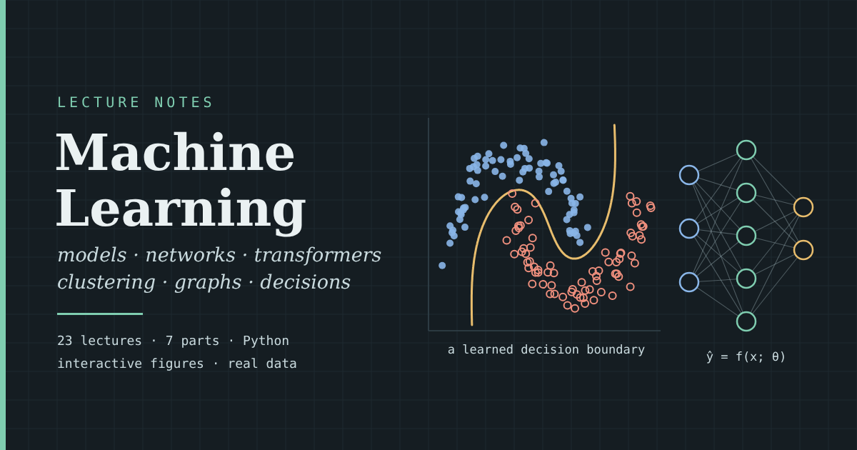
A visual, example-led course in machine learning for readers who know probability, statistics and some Python. Every lecture is one interactive page with intuition first, theorems with proofs, real data, Python code with its output, widgets to experiment with, and exercises and project ideas. By the end you can read current ML research papers.
Contents
- Lecture 1Learning from Data
Features, labels, loss and risk; k-nearest neighbours; overfitting and cross-validation; a first look at bias and variance; the Bayes-optimal predictor.
- 1.1 What problem are we solving?
- 1.2 Loss, risk and empirical risk minimisation
- 1.3 A first learner: k-nearest neighbours
- 1.4 Overfitting, validation and cross-validation
- 1.5 A first look at bias and variance
- 1.6 The best anyone could do: the Bayes-optimal predictor
- 1.7 Prediction is not explanation
- 1.8 Summary, exercises, projects, reading
Vectors and projections, eigenvectors and the SVD, gradients and Hessians, and the optimisers from gradient descent to Adam.
- 2.1 Data as vectors
- 2.2 Projection: the closest point on a line
- 2.3 Matrices are maps
- 2.4 Eigenvectors and the spectral theorem
- 2.5 The singular value decomposition
- 2.6 Calculus in many variables
- 2.7 Walking downhill: gradient descent, line search, momentum, Newton and Adam
- 2.8 Summary, exercises, projects, reading
- Lecture 3Linear Methods I: Regression
Least squares as projection, regression as maximum likelihood, ridge and lasso, Bayesian regression, and why coefficients are not causal effects.
- Lecture 4Linear Methods II: Classification
The perceptron, logistic and softmax regression, naive Bayes and LDA, and how to evaluate a classifier.
- 4.1 Drawing a line between classes
- 4.2 The perceptron
- 4.3 Logistic regression
- 4.4 More than two classes: softmax regression
- 4.5 Generative classifiers: discriminant analysis and naive Bayes
- 4.6 Evaluating a classifier
- 4.7 Propensity scores: classification for causal inference
- 4.8 Summary, exercises, projects, reading
What a loss encodes, surrogates and proper scoring rules, and the bias–variance decomposition computed exactly.
- 5.1 What a loss encodes
- 5.2 Regression losses and what they estimate
- 5.3 Losses from likelihoods
- 5.4 Classification: the 0–1 loss and its surrogates
- 5.5 Scoring probabilities: proper scoring rules
- 5.6 Bias and variance, precisely
- 5.7 Approximation, estimation, and choosing complexity
- 5.8 Losses you will meet later
- 5.9 Summary, exercises, projects, reading
Why training performance can predict test performance: PAC learning, VC dimension, Rademacher complexity and double descent.
- 6.1 The puzzle: why should training error mean anything?
- 6.2 One classifier: Hoeffding's inequality
- 6.3 PAC learning and finite classes
- 6.4 No free lunch
- 6.5 Infinite classes: shattering and VC dimension
- 6.6 Rademacher complexity: fitting pure noise
- 6.7 Linear classes, margins and Lipschitz losses
- 6.8 Modern puzzles: double descent, benign overfitting, PAC-Bayes
- 6.9 Summary, exercises, projects, reading
- Lecture 7Kernels and Support Vector Machines
Margins, duality and the SVM, the kernel trick, kernel ridge regression and Gaussian processes.
- 7.1 The widest street
- 7.2 Constrained optimisation: Lagrange multipliers, duality and KKT
- 7.3 The dual SVM, support vectors and soft margins
- 7.4 Feature maps and the kernel trick
- 7.5 Which functions are kernels?
- 7.6 The representer theorem and kernel ridge regression
- 7.7 Gaussian processes
- 7.8 Kernels at scale, in deep learning and on quantum computers
- 7.9 Summary, exercises, projects, reading
Decision trees, bagging and random forests, AdaBoost, gradient boosting and XGBoost, SHAP, and causal forests.
- 8.1 Trees as graphs
- 8.2 Growing a tree: impurity, greedy splits, pruning
- 8.3 Why one tree is not enough
- 8.4 Bagging and random forests
- 8.5 Boosting I: AdaBoost
- 8.6 Boosting II: gradient boosting
- 8.7 XGBoost and its relatives
- 8.8 Why trees still win on tables
- 8.9 Opening the black box: Shapley values and SHAP
- 8.10 Bayesian trees and causal forests
- 8.11 Summary, exercises, projects, reading
Graphs between data points: the graph Laplacian, label propagation, PageRank and graph neural networks.
- 9.1 Encoding graphs
- 9.2 From data to graphs
- 9.3 The graph Laplacian and smoothness
- 9.4 Spectra of graphs: what the eigenvectors look like
- 9.5 Semi-supervised learning: harmonic functions and label propagation
- 9.6 Random walks, diffusion and PageRank
- 9.7 Graph neural networks: learnable propagation
- 9.8 Graph-level tasks and the limits of message passing
- 9.9 Summary, exercises, projects, reading
- Lecture 10aNeural Networks I: What Networks Compute
Shallow and deep ReLU networks as piecewise-linear functions, activation functions, depth and universal approximation.
- Lecture 10bNeural Networks II: Training Them
Backpropagation by hand and by autodiff, initialisation, optimisers and regularisation for networks.
Shattered gradients, residual connections and normalisation, convolutional networks, and recurrent networks with LSTMs.
- 11.1 Why depth is hard: shattered gradients
- 11.2 Residual connections
- 11.3 Normalisation
- 11.4 Convolution: a sliding pattern detector
- 11.5 Pooling, invariance and receptive fields
- 11.6 Convolutional networks in practice
- 11.7 Recurrent networks and the gradient through time
- 11.8 LSTMs at work: forecasting and writing
- 11.9 The limits of recurrence, and its return
- 11.10 Summary, exercises, projects, reading
- Lecture 12Encoders, Attention and Transformers
Embeddings, self-attention, the transformer block, tokenisation, decoding strategies and retrieval-augmented generation.
- 12.1 Representing words
- 12.2 Encoders, decoders and the bottleneck
- 12.3 Attention: soft dictionary lookup
- 12.4 Multi-head attention and positions
- 12.5 The transformer
- 12.6 BERT, GPT and a tiny GPT of our own
- 12.7 Tokenisation: byte-pair encoding
- 12.8 Decoding: from probabilities to text
- 12.9 Pre-training, in-context learning and scale
- 12.10 Transformers in systems: retrieval and RAG
- 12.11 Summary, exercises, projects, reading
- Lecture 13Sentiment and Bias Analysis
Sentiment classifiers, bias in word embeddings, fairness criteria and the impossibility theorems, and a real audit.
- 13.1 Sentiment as classification
- 13.2 Lexicons, learned models and domain shift
- 13.3 Pre-trained representations
- 13.4 Bias in word embeddings
- 13.5 From representations to decisions
- 13.6 Fairness criteria
- 13.7 The impossibility theorems
- 13.8 Auditing the Lecture 8 income model
- 13.9 Causal notions of fairness
- 13.10 Summary, exercises, projects, reading
- Lecture 14Learning Without Labels
Density estimation, the curse of dimensionality, anomaly detection, Hopfield networks and self-supervised learning.
- 14.1 What "structure" means
- 14.2 Histograms and kernel density estimation
- 14.3 The curse of dimensionality
- 14.4 Anomaly detection
- 14.5 Energy-based models: Hopfield networks and Boltzmann machines
- 14.6 Self-supervised learning: inventing labels from the data
- 14.7 Evaluating without ground truth
- 14.8 Summary, exercises, projects, reading
- Lecture 15Clustering
k-means and k-means++, choosing k, hierarchical and density-based clustering, spectral clustering, and Kleinberg's impossibility theorem.
- Lecture 16aDimension Reduction I: Linear Methods
PCA and the SVD, eigenfaces, probabilistic PCA, random projections and matrix factorisation for recommendations.
- Lecture 16bDimension Reduction II: Nonlinear Methods
MDS, Isomap, Laplacian eigenmaps, t-SNE and UMAP, and autoencoders and VAEs.
- Lecture 17aMixture Models and EM
Gaussian mixtures and the EM algorithm, the ELBO, Dirichlet processes, hidden Markov models and topic models.
- 17a.1 Gaussian mixtures
- 17a.2 The EM algorithm
- 17a.3 Why EM works
- 17a.4 How many components? BIC and label switching
- 17a.5 Bayesian mixtures and the Dirichlet process
- 17a.6 Mixtures in time: hidden Markov models
- 17a.7 Mixtures of words: topic models
- 17a.8 Variational inference, and the VAE revisited
- 17a.9 Summary, exercises, projects, reading
- Lecture 17bCopulas: Dependence Beyond Correlation
Sklar's theorem, rank correlations and tail dependence, copula families, synthetic tabular data and the nonparanormal.
- 17b.1 Dependence beyond correlation
- 17b.2 Sklar's theorem: separating margins from dependence
- 17b.3 Measuring dependence with copulas: ranks and tails
- 17b.4 Copula families, fitting, and joint crashes
- 17b.5 Copulas in machine learning I: synthetic tabular data
- 17b.6 Copulas in machine learning II: the nonparanormal
- 17b.7 Summary, exercises, projects, reading
- Lecture 18Signal Processing and Spectral Analysis
The DFT and FFT, sampling and aliasing, filtering, spectral estimation, spectrograms, wavelets and matched filtering.
- 18.1 Sinusoids and roots of unity
- 18.2 The discrete Fourier transform and the FFT
- 18.3 Sampling and aliasing
- 18.4 Convolution and filtering
- 18.5 Spectral estimation: periodograms, Welch and windows
- 18.6 Time and frequency together: spectrograms and uncertainty
- 18.7 Wavelets
- 18.8 Matched filtering and the first gravitational wave
- 18.9 Summary, exercises, projects, reading
- Lecture 19Image Learning and Sound Learning
CNNs and symmetry, transfer learning and CLIP, diffusion as denoising, and learning from spectrograms.
- 19.1 Images as tensors; hand-designed features
- 19.2 CNNs through the Fourier lens; augmentation as symmetry
- 19.3 Transfer learning
- 19.4 Vision transformers, CLIP and zero-shot classification
- 19.5 Generative image models: diffusion as denoising
- 19.6 Sound: spectrograms, the mel scale and MFCCs
- 19.7 Audio classification
- 19.8 Speech recognition at scale
- 19.9 Summary, exercises, projects, reading
Correlation networks, graphs from smooth signals, Gaussian graphical models and the graphical lasso.
DAGs and d-separation, Markov equivalence, the PC algorithm, GES, NOTEARS and interventions.
The agent–environment loop, bandits and regret, off-policy evaluation, MDPs, Bellman equations and dynamic programming.
Monte Carlo and TD learning, n-step returns, SARSA and Q-learning, the deadly triad and DQN.
The policy gradient theorem, actor–critic and GAE, TRPO and PPO, Soft Actor-Critic, MCTS and offline RL.
- 22a.1 Why optimise policies directly
- 22a.2 The policy gradient theorem, REINFORCE and baselines
- 22a.3 Actor–critic and generalised advantage estimation
- 22a.4 Trust regions: TRPO and PPO
- 22a.5 Maximum-entropy RL and Soft Actor-Critic
- 22a.6 Planning with search and models
- 22a.7 Offline RL and off-policy evaluation
- 22a.8 Summary, exercises, projects, reading
Reward models from preferences, RLHF and DPO, GRPO and verifiable rewards, and reward hacking.
- Lecture 23Reading the Frontier
The anatomy of an ML paper, a notation decoder, reading experiments critically, and guided dissections of three papers.